1 Rey Reza Wiyatno & Liam Paull are with Montreal Robotics and Embodied AI Lab (REAL) & DIRO at the University of Montreal, and Mila
2 Anqi Xu conducted this work with support from his past affiliation with Element AI
Abstract: Commonly, learning-based topological navigation approaches produce a local policy while preserving some loose connectivity of the space through a topological map. Nevertheless, spurious or missing edges in the topological graph often lead to navigation failure. In this work, we propose a sampling-based graph building method, which results in sparser graphs yet with higher navigation performance compared to baseline methods. We also propose graph update strategies that eliminate spurious edges and expand the graph as needed, which improves lifelong navigation performance. Unlike controllers that learn from fixed training environments, we show that our model can be fine-tuned using only a small number of collected trajectory images from a real-world environment where the agent is deployed. We demonstrate successful navigation after finetuning on real-world environments, and notably show significant navigation improvements over time by applying our lifelong graph update strategies.
This page is dedicated to showcase our experimental results. For explanation about how our method works and other implementation details, please see our blog page.
Experimental Results
We use Gibson to quantify navigation performance in simulation. As for the robot, we use the LoCoBot in both simulated and real-world experiments, and we teleoperate it in each test map to collect trajectories for building the graph. We evaluate navigation performance to reflect real-world usage: the agent should be able to navigate between any image pairs from the graph, and should not just repeat trajectories based on how the images were collected.
Navigation Performance in Simulation
In this section, we compare the navigation performance of our method against SPTM and ViNG in the simulated environments. In this set of experiments, note that we do not perform graph updates with our method, which is evaluated separately under "Lifelong Improvement" section.
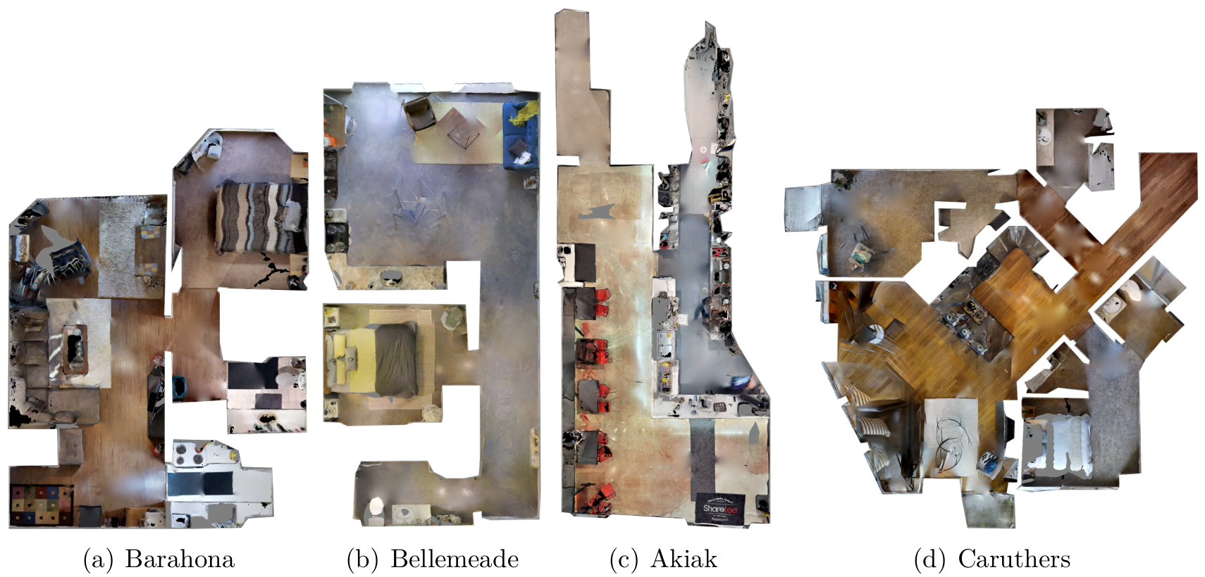
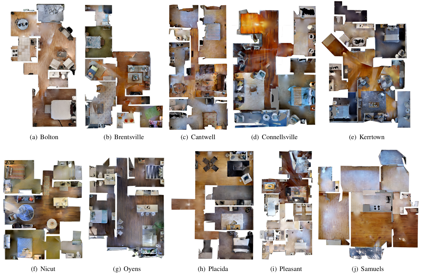
Fig. 1. Top-down view of the test environments (not to scale).
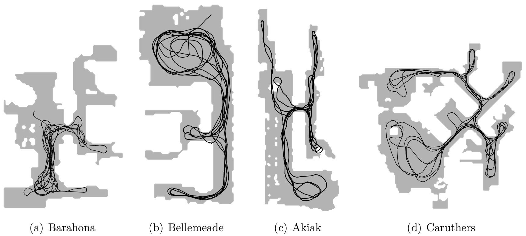
We evaluate on four test environments that are different from the model's training maps: Barahona (57m2), Bellemeade (70m2), Akiak (124m2), and Caruthers (129m2). These environments are shown in Fig. 1. For the graph building phase, we teleoperate the robot to explore roughly 3-4 loops around each map. Fig. 2 visualizes the top-down view of each test environment with its corresponding trajectory. We then pick 10 goal images spanning major locations in each map and generate 500 random test episodes. Since our graph building method is stochastic, we evaluate our method three times per environment.
Fig. 2. Top-down view of the agent's trajectory in each simulated test environment during trajectory collection phase (not to scale).
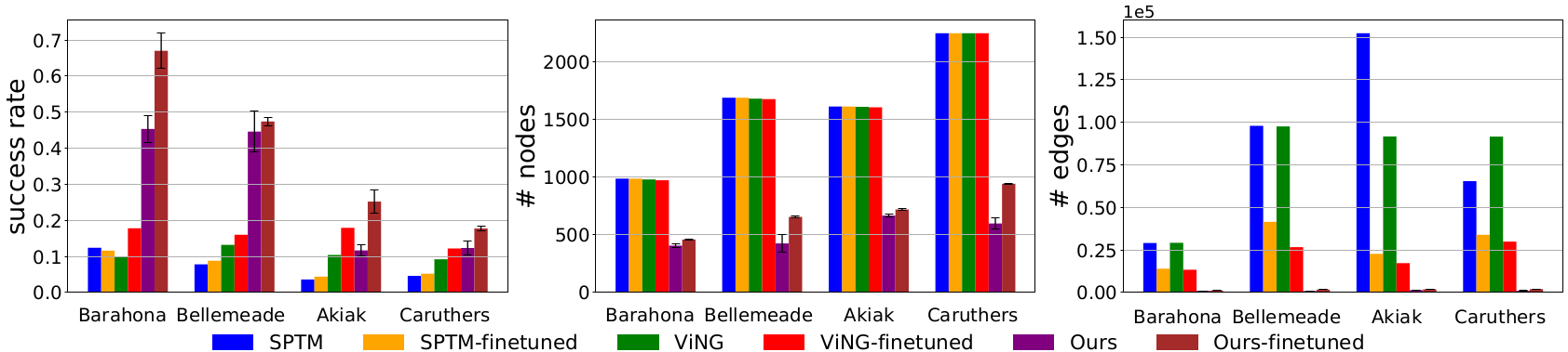
As seen in Fig. 3, our method consistently yields higher navigation success rates in all test environments when the model is fine-tuned. We can also observe that the performance gain of our model after fine-tuning is generally higher than others. Additionally, our graphs have significantly fewer number of nodes and edges, which keeps planning costs practical when scaling to large environments. Therefore, compared to the baselines that use entire trajectory datasets to build graphs, our sampling-based graph building method produces demonstrably superior performance and efficiency.
Fig. 3. Comparison of navigation success rates and graph sizes among topological visual navigation methods in various test environments.
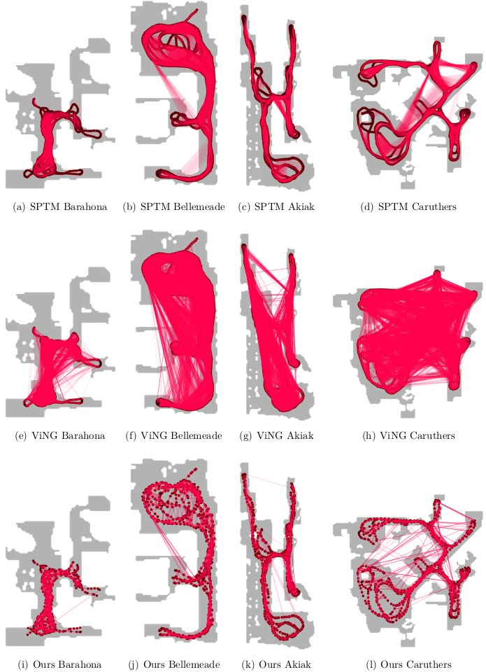
Fig. 4 qualitatively compares sample graphs built using different methods. We see that our graph has the fewest vertices, yet still maintains proper map coverage.
Visually, our graph also has few false-positive edges through walls, and we shall later demonstrate how our graph updates can further prune these.
Fig. 4. Comparison of the graphs built after model finetuning. Even without applying the graph updates, our method naturally produces a sparser graph.
Lifelong Improvement
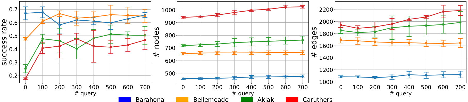
We now evaluate the proposed graph update method to see how navigation performance is affected as the agent performs more queries. We start these experiments using graphs built with our finetuned models. We then ask the agent to execute randomly sampled navigation tasks while performing continuous graph updates. After every 100 queries, we re-evaluate the navigation performance on the same static set of test episodes used in "Navigation Performance in Simulation" section.
Fig. 5. Changes in success rate, number of nodes, and number of edges as the agent performs more queries and update its graph in each test environment.
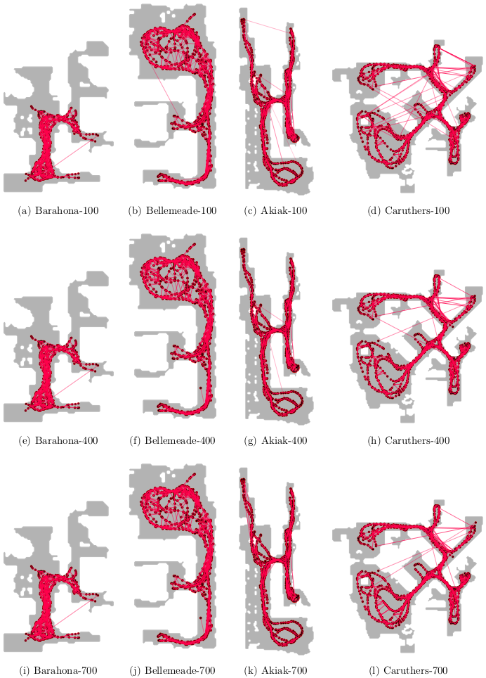
As seen in Fig. 5, the success rate generally improves as we perform more queries, with notable gains initially, while the number of nodes and edges in the graph do not substantially grow. We also see an initial decrease in the number of edges, suggesting that our graph updates successfully pruned spurious edges causing initial navigation failures, then later added useful new nodes for better navigation. Qualitatively, we can see fewer spurious edges when comparing sample graphs before and after updates in Fig. 6. We observe that sometimes the success rate decreased after a batch of graph updates. This is likely caused by spurious edges when adding new graph nodes near each 100th query, before we re-evaluate navigation performance. Nevertheless, such spurious edges are pruned in later updates, thus leading to increasing performance trends during lifelong navigation.
Fig. 6. Comparison of the updated graphs after executing 100, 400, and 700 navigation queries. We can see a notable reduction in spurious edges, especially ones that are across walls, which improved navigation performance in our experiments.
Below are some navigation videos from the simulated environments:
Real-world Experiments
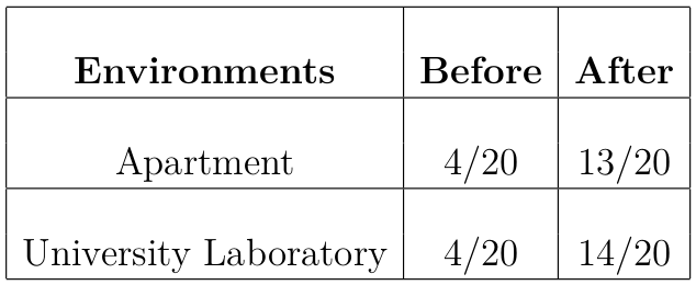
We evaluate the performance of our method in two real-world environments: a studio apartment and a medium-sized university laboratory. In Table 1, we report navigation success rates before and after we perform graph updates with 30 queries. These experiments confirm that our model performs well without needing large amounts of real-world data, especially when combined with our proposed lifelong graph maintenance, which enhances the navigation performance with more than 3x increase in success rate in both environments.
Table 1. Navigation success rate before and after graph updates in real-world environments.
Below are some navigation videos from the real-world environments:
Appendix
Model Architectures
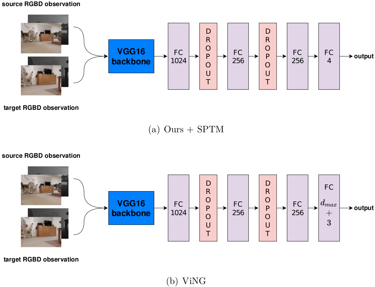
We present the model architecture that we used in our experiments.
Fig 7. Neural network architectures that we use in our experiments.
Training Environments
Here, we show the top-down view of environments we used to generate training dataset.
Fig. 8. Top-down view of the training environments (not to scale).
Navigation Parameters
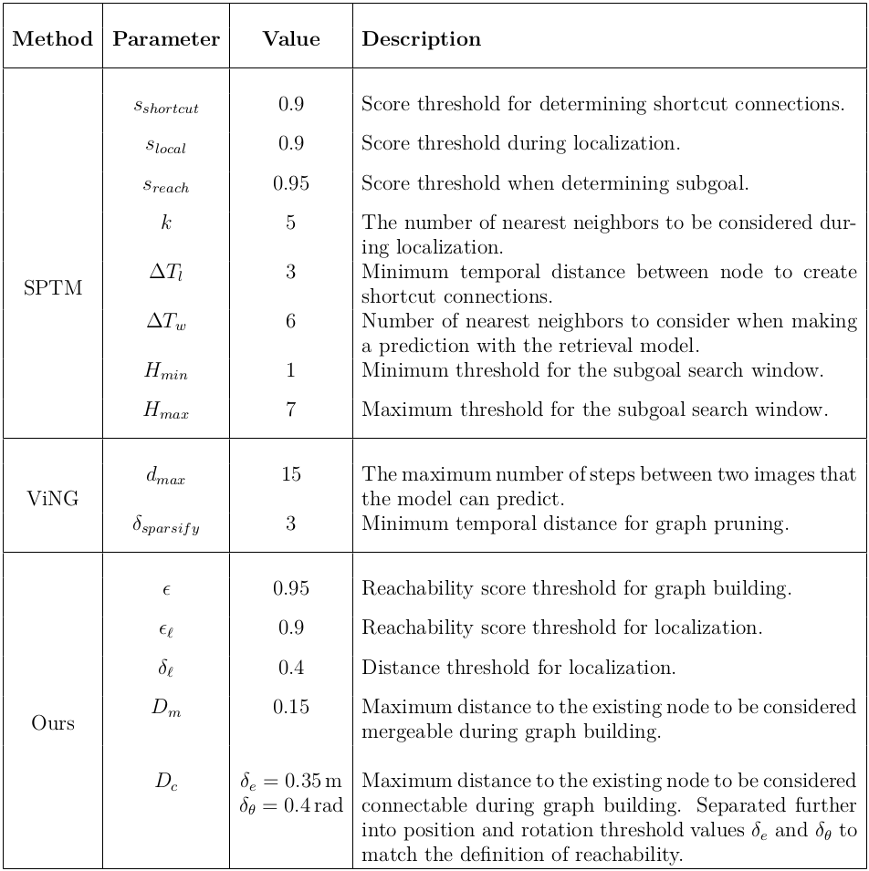
The parameters that we use in our experiments are shown in Table 2.
Table 2. Navigation parameters for each method.
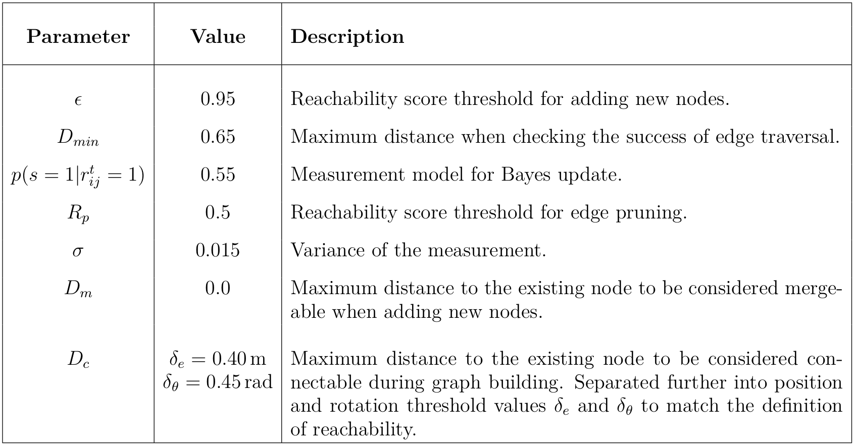
Additionally, the parameters that we use "Lifelong Improvement" experiments are shown in Table 3.
Table 3. Graph update parameters.
Additional Results
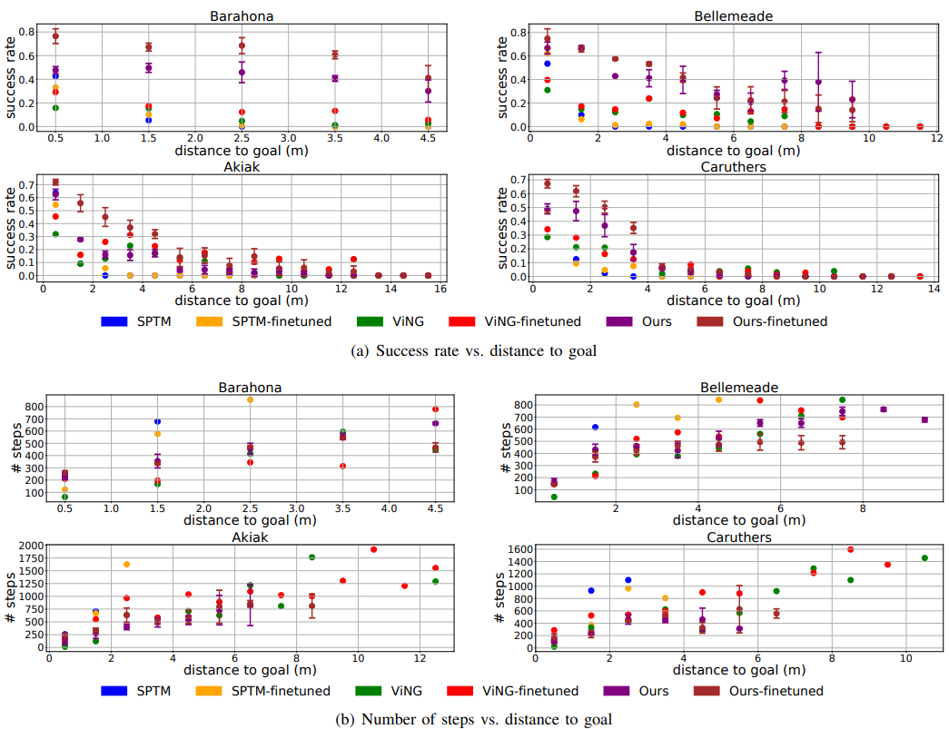
Here, we plot success rate and number of steps required as the geodesic distance to goal changes in each test simulated environment.
Fig 9. Plots of success rate and number of steps required as the geodesic distance to goal changes in each test simulated environment.
 |
|
 |
|