When we talk about robot navigation, we usually think about building a metric map of the environment using SLAM techniques. However, with this type of metric-based navigation, it is unintuitive to specify goals in metric space, and also tedious for an expert user to pilot the robot around to build the map. Ideally, navigation goals should carry semantic meaning that we can comprehend easily, such as images of target objects or locations. Imagine if we just bought a robot for our home and want this robot to navigate to a particular location. We probably do not want to enter a numerical coordinate to interact with the robot, do we? Instead, as illustrated in Fig. 1, picking a previously taken image from the memory (e.g., picture of our kitchen) as the target for the robot is arguably more intuitive for us.
Fig. 1. Illustration of a possible navigation interface with image goals. All we need to do is pick an image as a navigation goal for the robot.
Another class of approaches is end-to-end learning-based methods that directly map image inputs to actions. Nevertheless, these policies tend to be reactive and are not suitable for long-distance navigation. While RL can be considered as the frontrunner in this class of approaches, training RL policies requires significant computation and time, and thus is impractical to do in real-world environments. Furthermore, when trained in simulation, these models do not usually transfer well to the real-world.
In our work, we are interested in another type of map called topological map which is represented as a graph. In such a setup, each edge in the graph encodes the traversability between two locations, while a local controller is used to actually navigate the edge. As a result we can decompose a possibly long-distance navigation query into shorter ones via graph planning. In contrast to a global controller, navigating within a local vicinity is a much easier task than navigating globally through a complex environment layout. The challenge here is how to construct such a representation in an efficient way that enables a local controller to navigate the environment.
In our case, the nodes in our graph correspond to RGBD images of particular locations from an environment. We develop a model that jointly predicts reachability and relative transformation between two RGB-D images, which we will use to determine connectivity between the nodes of the graph. Importantly, we show that this model can be pre-trained using automatically generated simulated data, and then fine-tuned using only the data that is collected to build the graph in the target environment.
To build the graph, we take inspiration from traditional sampling-based robotics planners such as probabilistic roadmaps (PRM) and rapidly-exploring random trees (RRT) but formulate the problem over sensor data space rather than configuration space. We propose a sampling-based graph building process that produces sparser graphs and also improves navigation performance when compared to baselines. We construct this graph by sampling nodes from a pool of collected images and using our model to determine the connectivity between the nodes.
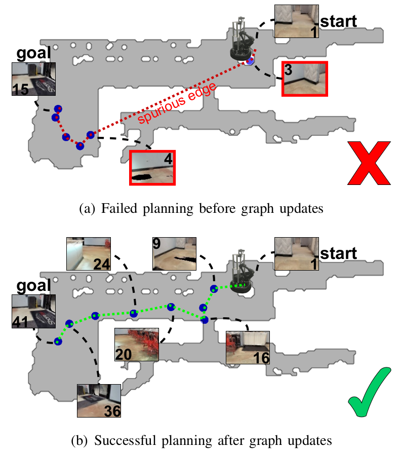
Since the connectivity of our graph is determined by querying a potentially imperfect predictive model, it is important to address the possibility of spurious edges. False positives from this model will induce spurious edges in the graph and may cause the agent to execute infeasible plans, while false negative predictions will result in edges being omitted and may result in failure to find a path when one actually exists. Thus, while other methods treat their graphs as static objects, we continually refine ours based on what our agent experiences when executing navigation queries. These graph updates eliminate spurious edges and possibly add new nodes that might be missing, as shown in Fig.2, which improves navigation performance over time.
Fig. 2. Sample plans produced with our method to navigate from a start to a goal image before and after graph updates. The blue dots indicate the nodes within the planned path. The plan in Fig. 2(a) led to navigation failure since nodes #3 and #4 are mistakenly connected. Fig. 2(b) showcases the new plan that we obtained after performing our proposed graph updates which led to successful navigation. This demonstrates how our graph updates successfully refined the graph by removing the spurious edge.
To summarize, our main contributions are:
A sampling-based graph building process that produces sparser graphs and improves navigation performance,
A multi-purpose model for graph building, path execution, and graph maintenance, that can be fine-tuned in real-world using small amount of data,
A graph maintenance procedure that improves lifelong navigation performance.
Proposed Method
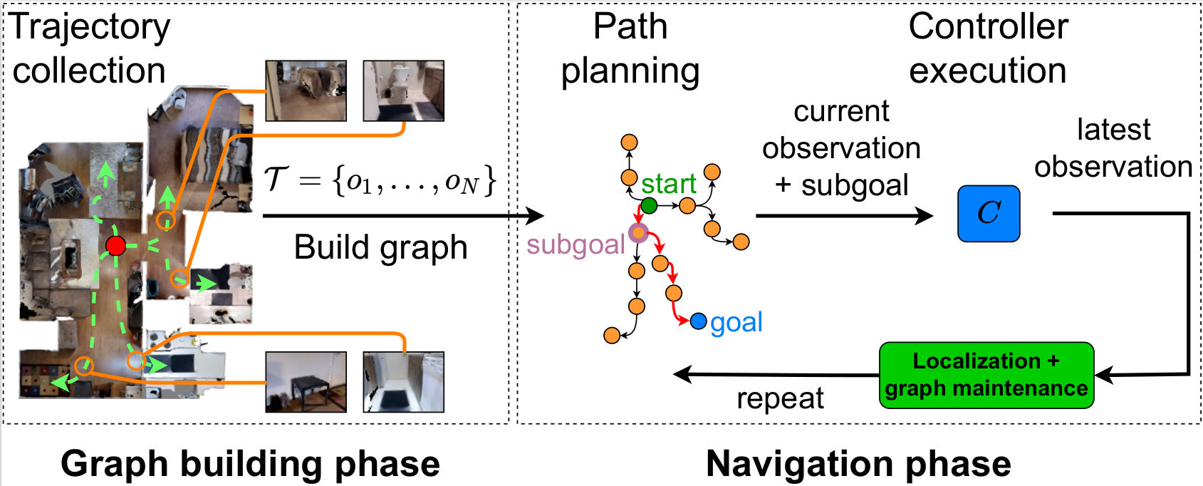
We focus our work on visual navigation tasks where the goal is specified by a target RGB-D image. Fig. 3 below illustrates the navigation framework that we are working with. When we deploy our agent in a target environment, we first execute a trajectory collection phase to obtain a pool of RGBD images \(\mathcal{T} = \{o_1, ..., o_N\}\). We then use \(\mathcal{T}\) to build a graph \(G=(V,E)\), where vertices \(V\) are a subset of the collected images, and directed edges \(E\) represent traversability (we will discuss later how we define traversability).
During navigation, we present the agent with a query represented as an RGBD goal image \(o_{g}\). The agent first localizes itself on the graph based on its current observation \(o_{c}\), and plans a path to reach \(o_{g}\).
From the planned path, the agent picks a subgoal observation \(o_{sg}\) and moves towards it using its controller.
After executing the control command, the agent relocalizes itself on the graph using its latest observation, and updates the graph based on its experience. These processes are repeated until the agent reaches \(o_g\).
Fig. 3. A common topological navigation framework consists of separate graph building and navigation phases. When deployed in a new environment, an agent first collects observations from an environment and builds a topological graph. During navigation, the agent localizes itself on the graph, plans a path to a given goal, and moves to a subgoal using a controller. The agent then relocalizes itself, and repeats the planning and control steps until it reaches the goal. Our work highlights the importance of updating the graph, which is missing from most existing work.
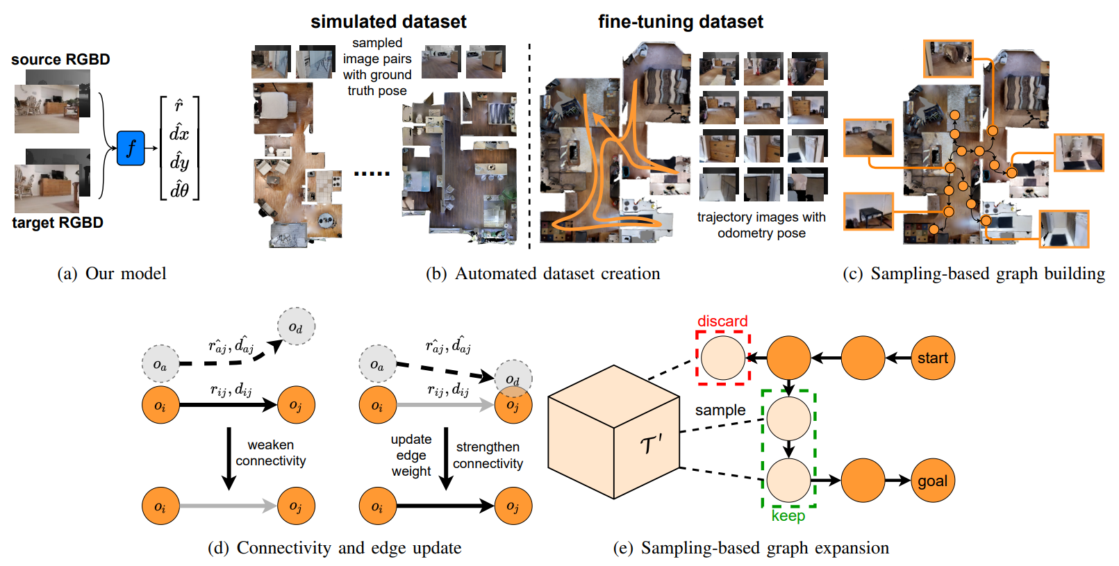
The rest of this section discusses our main contributions, which are illustrated in Fig. 4. First, we present our simple yet versatile model that is the crux of our navigation system, be it for graph building, path execution, or graph updates. We then discuss our proposed sampling-based graph building algorithm that produces sparser graphs compared to baselines, and how to perform navigation with our model. Finally, we present lifelong graph maintenance strategies that lead to increases in navigation performance as our agent executes more queries in a target environment.
Fig. 4. Illustrations of our main contributions. Fig. 4(a) depicts the proposed model, which takes source and target RGB-D images and outputs a reachability score \(\hat{r}\) and a waypoint \(\hat{w} = [\hat{dx}, \hat{dy}, \hat{d\theta}]\). As shown in Fig. 4(b), we first train our model in simulation by collecting RGB-D image pairs from different environments. Later, we fine-tune our model in a new environment using only RGB-D images and their corresponding odometry data from a collected trajectory. Our sampling-based graph building method is depicted in Fig. 4(c), where we only select a portion of trajectory images to build the graph. Fig. 4(d) illustrates one of the proposed graph maintenance methods that updates the graph based on the success of an agent in traversing an edge. If the agent fails, the edge connectivity is weakened, else, its connectivity is strengthened and its weight is updated. Fig. 4(e) illustrates the second graph maintenance method that expands the graph by sampling from the remaining trajectory data \(\mathcal{T'}\) to enable planning when the agent is unable to find a path.
Reachability and Waypoint Prediction Model
Our goal is to design a model that we can use in most of the navigation aspects. We train a convolutional neural network \(f(o_i, o_j) = [\hat{r}, \hat{dx}, \hat{dy}, \hat{d\theta}]\) that takes two RGB-D images \((o_i, o_j)\) and jointly estimates reachability \(r \in \{0,1\}\) from one image to another, and their relative transformation represented as a waypoint \(w = [dx, dy, d\theta] \in \mathbb{R}^{2} \times (-\pi, \pi]\). To simplify the pose estimation problem, the waypoint only contributes to the training loss for reachable data points.
This model is used in a number of the components of our system. First, we use our model for graph building by using the reachability and pose estimates to determine the node connectivity and edge weights, respectively. We also use our model to perform localization, and the proposed graph updates. Furthermore, we use a position-based feedback controller to navigate to waypoints predicted by our model.
We train our model with full supervision in simulation on a broad range of simulated scenes by minimizing the binary cross-entropy for reachability and regression loss for the relative waypoint. Additionally, we can later fine-tune our model using only the trajectory data acquired from the environment where the agent is deployed. As a result, we can use our model in the real-world environment without needing to tediously collect and manually label a large amount of real-world data. We discuss how we create both simulated and fine-tuning datasets below.
Automated Dataset Creation
We aim to create a diverse dataset such that our model can generalize well to real-world environments without collecting a large real-world dataset. We thus create a dataset by sampling image pairs from various simulated environments.
In simulation, the waypoint label can be computed easily since the absolute pose of each observation is known. For reachability between two RGB-D observations, similar to Meng et al. (2020), we define node-to-node reachability to be controller-dependent. Nevertheless, instead of rolling out a controller to determine reachability, we assume a simple control strategy based on motion primitives (i.e., Dubins curves), which allows us to compute reachability analytically.
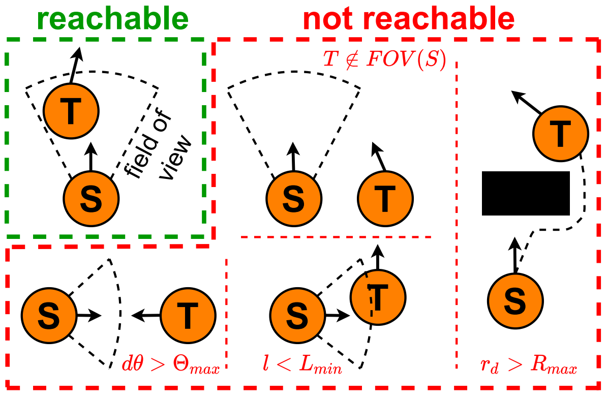
We determine the reachability label based on visual overlap and spatial distance between two observations. Fig. 5 illustrates various reachable and non-reachable situations during data collection in simulation. Specifically, two observations are labeled as reachable if:
The visual overlap ratio between the two images, \(l\), is larger than \(L_{min}\), computed based on depth data;
The ratio of the shortest feasible path length over Euclidean distance between the poses, \(r_{d}\), is smaller than \(R_{max}\), to filter out obstacle-laden paths;
The target pose must be visible in the initial image, so that our model can visually determine reachability;
The Euclidean distance to the target is less than \(E_{max}\), and the relative yaw is less than \(\Theta_{max}\).
In our experiments, we computed visual overlap by comparing point cloud data of each image pixel, which is available in the simulator that we use. This remains a secondary implementation detail, as we recognize that there are valid alternative approaches that can also be used to compute visual overlap depending on what information is available from a simulator.
Fig. 5. Illustration of reachable and non-reachable situations for a pair of source (S) and target (T) nodes.
During training, we define \(o_j\) to be reachable only if it is in front of \(o_i\). Yet, when navigating, the agent can move from \(o_j\) to \(o_i\) by following the predicted waypoint \(w\) in reverse.
A key feature of our method is the ability to fine-tune our model in the target domain, by using the same trajectories collected to build the graph. Although SPTM (Savinov et al., 2018) and ViNG (Shah et al., 2021) can be trained on target-domain trajectories, our model does not need to be trained on a large real-world dataset, as it has already been trained within various simulated environments. As an added requirement for real-world fine-tuning, the collected trajectories must have associated pose odometry to substitute for ground-truth pose data. Thankfully, odometry is readily available from commodity robot sensors such as inertial measurement units or wheel encoders.
Since visual overlap and shortest feasible path length are no longer accessible during fine-tuning, as a proxy criterion we take an observation pair \((o_i, o_j) \in \mathcal{T}\) where \(j > i\) and check if they are separated by at most \(H\) time steps during trajectory collection. The use of odometry as a supervisory signal for pose estimation can be noisy; however, since reachable waypoints must be temporally close, the long-term pose drift should be minimal.
Sampling-based Graph Building
A dense graph is likely to exhibit spurious edges and is the primary cause of failure in topological navigation or at best is inefficient to search over. Our goal is to build a graph with a minimum number of nodes and edges without sacrificing navigation performance. Thus, instead of using all images in \(\mathcal{T}\), we build our graph incrementally via sampling.
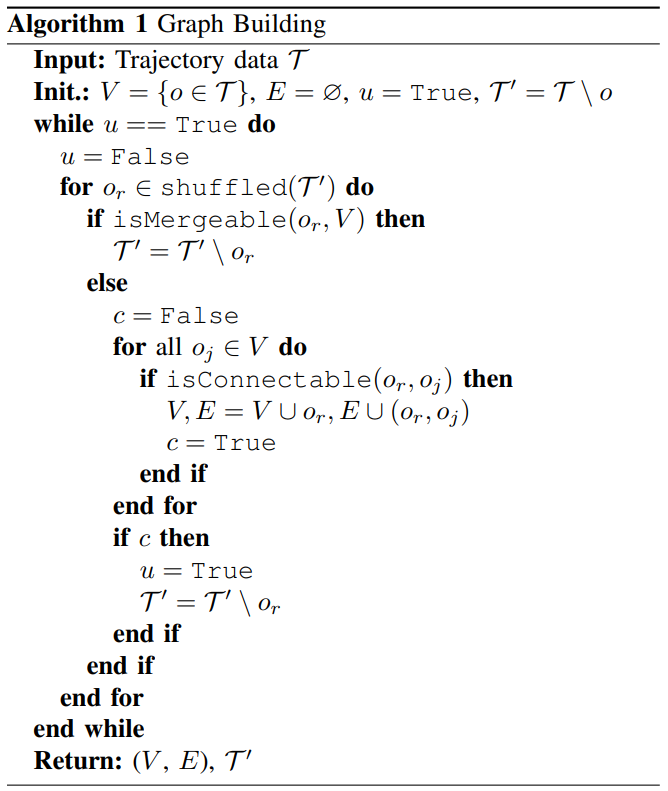
Algorithm 1 below describes the proposed graph building process.
We initialize the graph as a randomly drawn node \(o \in \mathcal{T}\). We also initialize a copy of the trajectory data \(\mathcal{T'} = \mathcal{T} \setminus o\) to keep track of nodes that are not yet added to the graph. Then, in each iteration, we sample a node \(o_{r} \in \mathcal{T'}\) (or equivalently, sampling from shuffled \(\mathcal{T'}\)), check if it can be merged with or connected to existing graph vertices, and if so, remove it from \(\mathcal{T'}\). If \(o_{r}\) can be connected with any of the existing nodes \(o_j \in V\), we weigh the edge with a distance function based on the relative pose transformation between the pair as predicted by the model \(f\). Concretely, we define the distance to a waypoint \(w\) as
\(d(w) = ||\log T(w)||_{F},\)
where \(T(\cdot)\) converts a waypoint into its matrix representation in \(SE(2)\), and \(||\cdot||_{F}\) computes the Frobenius norm. This procedure continues until no more nodes can be added.
To build a sparse yet reliable graph, we would like to connect nodes that are close together, but not the ones that are too close. To this end, we introduce two operators: \(\texttt{isMergeable}\) and \(\texttt{isConnectable}\). First, \(\texttt{isMergeable}\) assesses whether a node is excessively close to existing nodes and thus can be thrown away for being redundant. Second, \(\texttt{isConnectable}\) checks if a node is sufficiently close to another node such that a local controller can successfully execute the edge directly. These two distance thresholds are controlled by empirically-tuned hyperparameters \(D_m\) and \(D_c\). Due to the proposed node merging mechanism, our graph building method results in a sparser graph compared to other methods.
In practice, if we know how \(\mathcal{T}\) is collected, we can improve the efficiency of the algorithm by biasing the node sampling process. For example, we can increase the node sampling probability based on how far the remaining nodes are from each of the existing nodes in the graph. Also, we can further increase the flexibility of tuning parameters such as \(D_{m}\) and \(D_{c}\) by using separate position and rotation threshold values.
Navigation
Here, we describe how we can execute a navigation query with our model \(f\) and the graph \(G\) built using trajectory data from the test environment \(\mathcal{T}\). We first localize the agent on the graph based on its current observation \(o_a\). Concretely, we use \(f\) to compare pairwise distances between \(o_a\) and all nodes in the graph and identify the closest vertex where the distance is below \(D_{\ell}\). To save computational cost, we first attempt to localize locally by considering only directly adjacent vertices from nodes within the last planned path, and then reverting to global localization (i.e., considering all nodes) if this fails.
For planning, we use Dijkstra's algorithm to find a path from where \(o_a\) is localized to a given goal vertex \(o_g \in V\), and select the first node in the path as subgoal \(o_{sg}\). We then predict the waypoint from \(o_{c}\) to \(o_{sg}\), and use a position-based feedback controller to reach \(o_{sg}\). At the end of controller execution, we update \(o_a\) to be the latest observation, and relocalize the agent. Based on the latest observation, we perform our graph updates to refine the graph, as will be described later. These are then repeated until the agent arrives at \(o_g\).
Lifelong Graph Maintenance
We propose two types of continuous graph refinements to aid navigation performance. The first is a method to correct graph edges based on the success of an agent in traversing an edge. This results in the removal of spurious edges and enhanced connectivity of traversable edges. Second, we add new nodes to the graph either when observations are novel or when we cannot find a path to a goal.
We define two properties associated with each edge between physical locations \(i\) and \(j\) that are revised during graph maintenance: an edge's true connectivity after the \(t\)-th update modeled as \(r^t_{ij} \sim \textrm{Bernoulli}(p^t_{ij})\), and an edge's distance weight modeled as \(d^t_{ij} \sim \mathcal{N}(\mu^t_{ij}, (\sigma^t_{ij})^2)\). These are initialized respectively as \(p^0_{ij} = \hat{r}^0_{ij}\), \(\mu^0_{ij} = d(\hat{w}^0_{ij})\), and \((\sigma^0_{ij})^2 = \sigma^2\), where \((\hat{r}^0_{ij}, \hat{w}^0_{ij}) = f(o_i, o_j)\) are the predictions of our model during graph building, and \(\sigma^2\) is derived empirically from the variance of our model's distance predictions across a validation dataset. We further define the probability of successful traversal through an edge as \(p(s)\), where the conditional likelihood of the edge's existence \(p(s|r)\) is also empirically determined.
Fig. 4(d) depicts how we update these edge properties after each traversal attempt. Given the agent's observation \(o_a\) that is localized to \(o_i\) on the graph, a target node \(o_j\), the agent's latest observation after edge traversal \(o_d\), we determine success of traversal via \(\texttt{isConnectable}(o_d, o_j)\). We then update the edge's connectivity using discrete Bayes update:
When the agent fails to reach \(o_j\), we prune the edge when \(p(r^{t+1}_{ij}|s) < R_{p}\). Upon a successful traversal, we also use the predicted distance \(d(\hat{w}_{aj})\) between \(o_a\) and \(o_j\) to compute the weight posterior with Gaussian filter:
In this way we can correct for erroneous edges based on what the agent actually experiences during navigation.
To expand the graph, if an observation cannot be localized, we consider it as novel and add it to the graph. Separately, Fig. 4(e) depicts how we expand our graph when a path to a goal is not found during navigation. In this situation, we iteratively sample new nodes from the remaining trajectory data \(\mathcal{T'}\) until a path is found, and store them into a candidate set \(\tilde{V}\). Denoting the nodes within the path as \(V_p\), we then add only the new nodes that are along the found path \(\tilde{V} \cap V_p\) to the graph permanently and remove them from \(\mathcal{T'}\), while returning other nodes \(\tilde{V} \setminus (\tilde{V} \cap V_p)\) back into \(\mathcal{T'}\). When connecting a novel node to existing vertices, we loosen the graph building criteria by increasing \(D_c\), especially to accommodate adding locations around sharp turns. This is because the nodes in \(\mathcal{T'}\) by construction did not meet the original criteria of \(\texttt{isConnectable}\) during graph building.
Takeaways
We proposed a simple model that can be used in many aspects of the adopted topological navigation framework. Equipped with this model, we proposed a new image-based topological graph construction method via sampling, which not only produces sparser graphs compared to baselines, but also higher navigation performance. We also introduced a lifelong graph maintenance approach by updating the graph based on what our agent experiences during execution of navigation queries. We showed that these updates add useful new nodes and remove spurious edges, thus increasing lifelong navigation performance. We also demonstrated a training regime using purely simulated data, combined with fine-tuning using only the trajectory data from a target domain, which resulted in strong real-world navigation performance.
Below are some navigation examples both in simulation and real-world environments. To see more results, please visit our home page.
References
Nikolay Savinov, Alexey Dosovitskiy, Vladlen Koltun. Semi-parametric Topological Memory for Navigation. ICLR, 2018.
Xiangyun Meng, Nathan Ratliff, Yu Xiang, Dieter Fox. Scaling Local Control to Large-Scale Topological Navigation. ICRA, 2020.
Dhruv Shah, Benjamin Eysenbach, Gregory Kahn, Nicholas Rhinehart, Sergey Levine. ViNG: Learning Open-World Navigation with Visual Goals. ICRA, 2021.
 |
|
 |
|